| 2D Map | 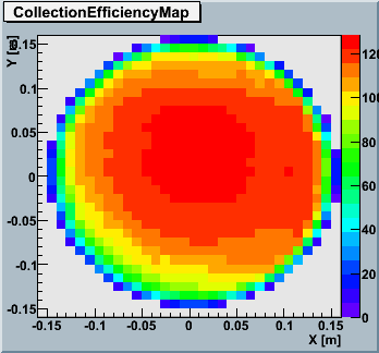 |
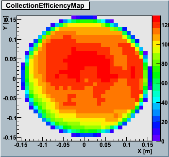 |
|---|---|---|
| PMT | averaged 94 PMTs | averaged all GoldenPMTs |
PMT 2D Correction Efficiency(CE) Maps are variety.
This analysis aim to understand CE average behavior.
So, we average all 94 PMT 2D Maps measured in Chiba for 3 year-long, or 16 Golden PMTs.
This table averaged all PMTs will be default of ROMEO.
| 2D Map |  |
 |
|---|---|---|
| PMT | averaged 94 PMTs | averaged all GoldenPMTs |
Average all 13 Golden DOMs convoluted QE average @337nm.
| 2005 | Dosetsu_Inuyama, Genpachi_Inukai, Kobungo_Inuta, Shinbei_Inue, Shino_Inuzuka |
|---|---|
| 2006 | BakeNeko, DorobohNeko, IeNeko, ManekiNeko NemuriNeko, NoraNeko, SuteNeko, YamaNeko |
| 2D Map | 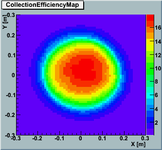 |
|---|---|
| DOM | averaged all Golden DOM |
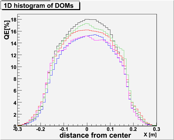
The two plots below shows sliced 2D map by axis, each PMT or DOM.
DOM 1D dist is convoluted QE @337nm, PMT is relative.
| 1D Hist | 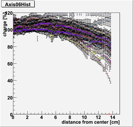 |
 |
|---|---|---|
| all PMTs | FY2006 GDOM @ 365nm (inspect ManekiNeko) |
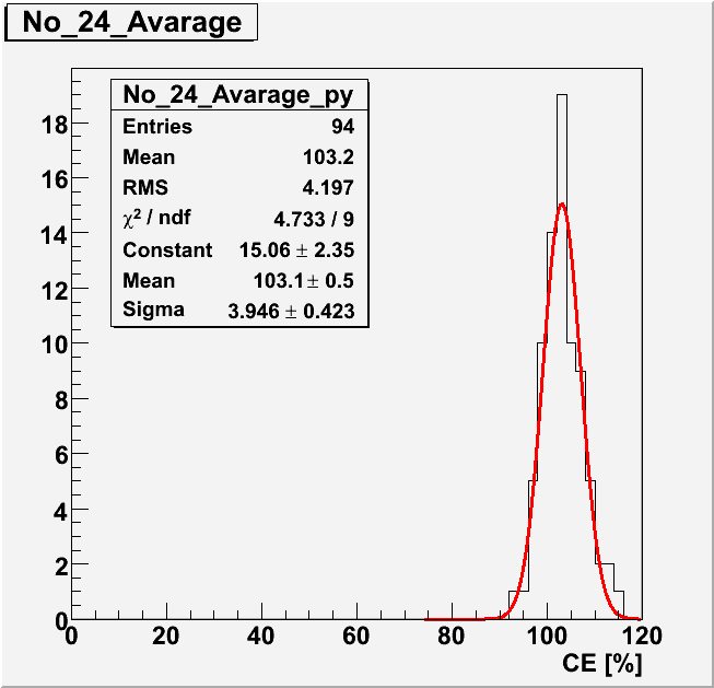
The plot below is distribution at 2.4cm point from center.
And calculate this mean each point for 2D averaged table.
 one axis distribution