 Contents
  Contents
  Introduction
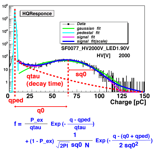
 The analytical function shown below has been used to represent the PMT charge response and implemented in the PMT simulation "ROMEO". The implementation was made when the calibration data was statistically limited, however. It is now over 4 years since Chiba started the PMT calibration and the present data is rich enough to picture "average" behavior of the IceCube PMT response. Here we describe the results of the systematic study on the charge response based upon the calibration data of 118 PMTs. The distributions of values of the coefficients in the analytical response function are plotted in various gains. We also build a hypothetical "average" IceCube PMT response model by averaging those values. This is to be implemented in ROMEO to represent the default IceCube PMT in the detector simulations.
See also.
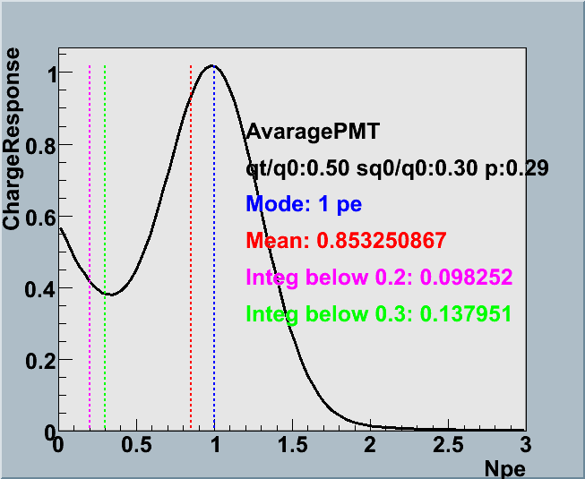
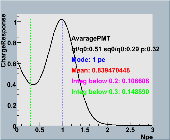
 Average of Charge Response
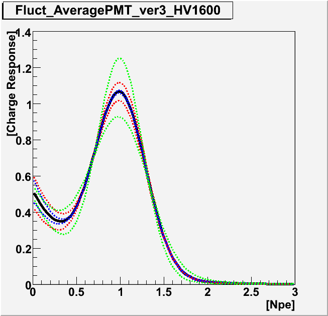
 Plotted below are the average charge response functions for three different gain settings. In order to see the fluctuation of the response function, the lower panels shows the curves of the function with the higher and lower values of the coefficients by 1 sigma. Red curves correspond to the case when pe is shifted by ±1 sigma. Blue for qtau/q0, green for sq0/q0.
| Average | 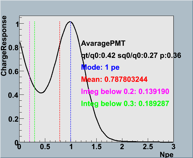 |
 |
 |
|---|---|---|---|
| Fluctuation | 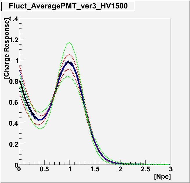 |
 |
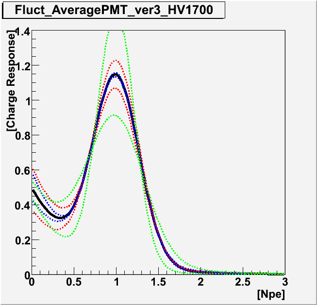 |
| Gain | 5.0e+7 | 7.0~8.0e+7 | 10.0~12.0e+7 |
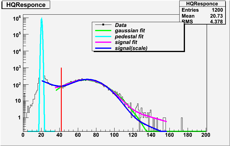
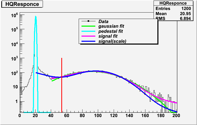
 An example of the charge histogram in the fitting (TA3753)
 | fitting histogram | 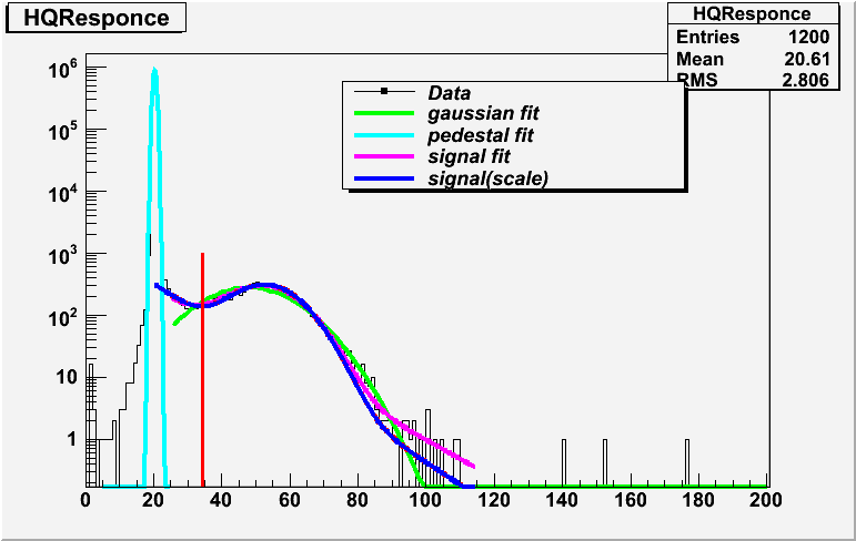 |
 |
 |
|---|---|---|---|
| gain | 5.0e+7 | 7.0~8.0e+7 | 10.0~13.0e+7 |
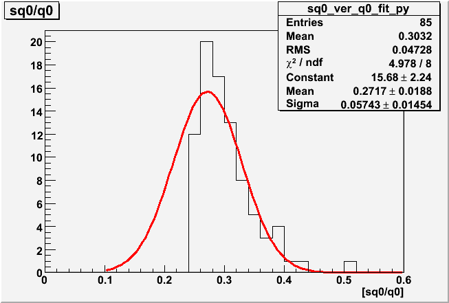
 Distribution of sq0/q0 obtained from the 118 PMTs
This parameter corresponds to the charge resolution of PMT. Most of an individual PMT has been measured in five different gains. It is found that no obvious gain dependences have been observed. This implies that the parameterization of the response function is valid in the gain range of the IceCube operation.
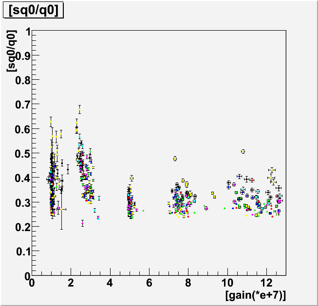 2D Graph : gain & sq0/q0 (3sigma cut)
Table1 [1D Histogram by projection of 2D Graphs in three groups of gain ]
| Histogram | 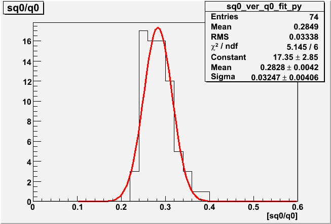 |
 |
 |
|---|---|---|---|
| Gain | 5.0e+7 gain | 7.0~8.0e+7 gain | 10.0~12.0e+7 gain |
| Average | 0.2828 ± 0.0095 | 0.2937 ± 0.0099 | 0.2717 ± 0.0204 |
| Sigma | 0.0325 | 0.0349 | 0.0574 |
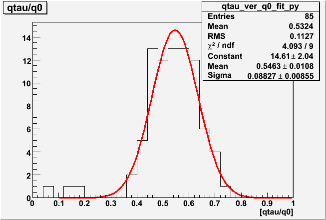
 Distribution of qtau/q0 obtained from 118 PMTs
"qtau" corresponds to decay time of exponential term of fit function
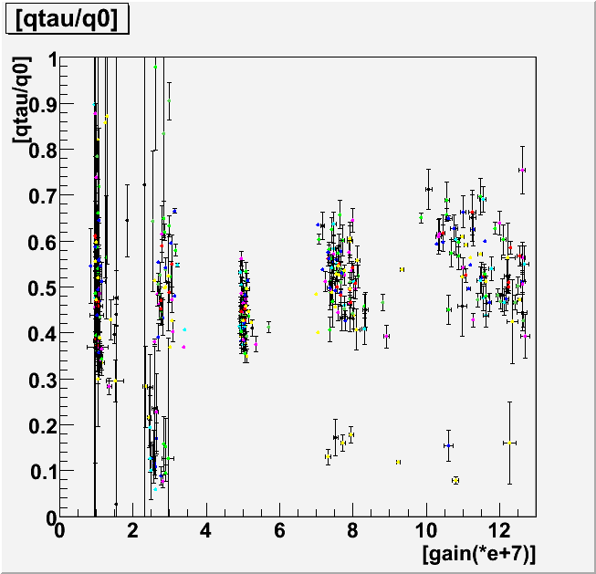 gain & qtau/q0(3sigma cut)
Table2 [1D Histogram by projection of 2D Graphs in three groups of gain ]
| Histogram | 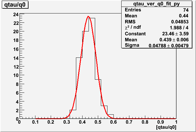 |
 |
 |
|---|---|---|---|
| Gain | 5.0e+7 gain | 7.0~8.0e+7 gain | 10.0~12.0e+7 gain |
| Avarage | 0.4390 ± 0.0144 | 0.5226 ± 0.0172 | 0.5463 ± 0.0196 |
| Sigma | 0.0479 | 0.0645 | 0.0883 |
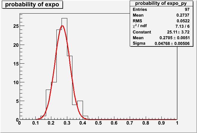
 Distribution of pe obtained from 118 PMTs
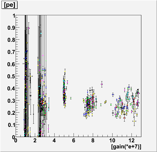 gain & pe (5sigma cut)
Table3 [1D Histogram by projection of 2D Graphs in three groups of gain ]
| Histogram | 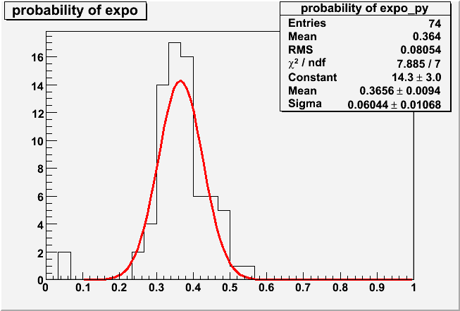 |
 |
 |
|---|---|---|---|
| Gain | 5.0e+7 gain | 7.0~8.0e+7 gain | 10.0~12.0e+7 gain |
| Avarage | 0.3656 ± 0.0095 | 0.2705 ± 0.0096 | 0.2719 ± 0.0090 |
| Sigma | 0.0604 | 0.0477 | 0.0676 |
 Why we should NOT use parameter values obtained at the low gain (< 3e+7) data?
| sq0/q0 |  |
 |
|---|---|---|
| qtau/q0 | 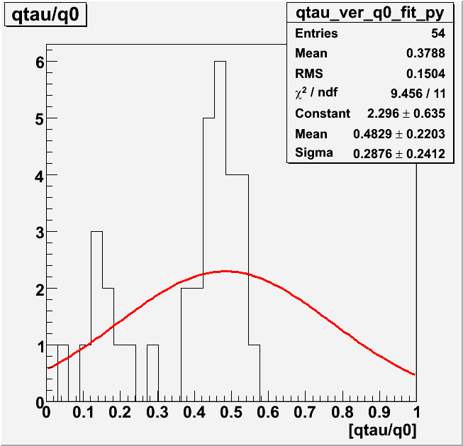 |
 |
| pe | 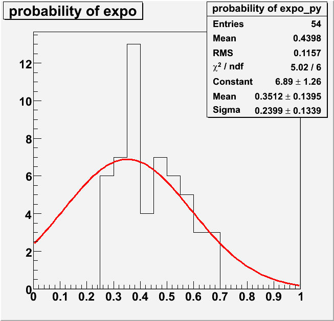 |
 |
| Gain | 2.0~3.0e+7 | 5.0+7 |
 Conclusion
Charge Response can be described in PMT gain independent way within our resolution of the present measurements. For the reference, shown below is the average charge response function curve in comparison with the 2006 ROMEO default model.
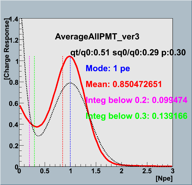 Difference of Average and ROMEO
Red solid line : AVERAGE charge response all PMT (>5e+7 gain)
Black dotted line : ROMEO charge response
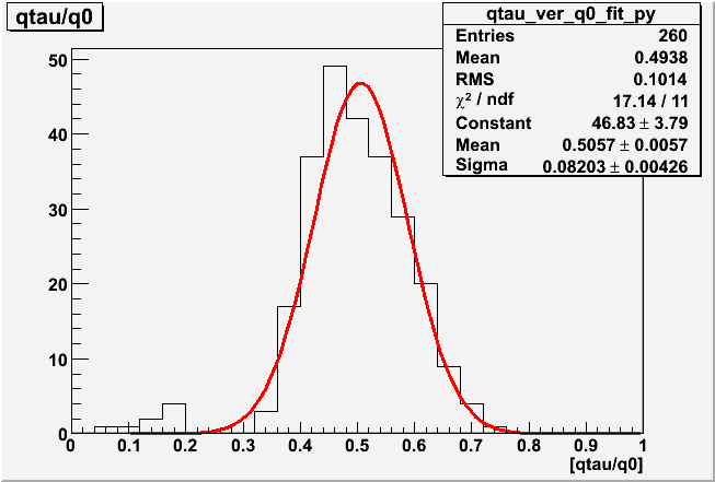
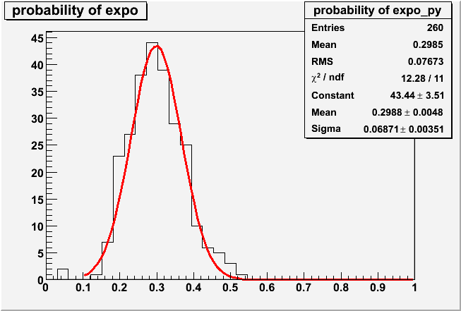
Table4 [1D Histogram by projection of 2D Graphs (>5e+7 gain) ]
| Histogram |  |
 |
 |
|---|---|---|---|
| Parameter | sq0/q0 | qtau/q0 | pe |
| Avarage | 0.2916 ± 0.0091 | 0.5057 ± 0.0162 | 0.2987 ± 0.0102 |
| ROMEO | 0.3650 | 0.1219 | 0.2765 |