Linearity measurement and Pre-, After- and Latepulses
Rationale
When very many photons arrive at the photocathode in a short time, saturation effects, mainly from the base components can arise. This measurement aims to characterize the behavior of DEgg PMTs to such large charges. This also comes with a measurement of prepulses, afterpulses, and latepulses.
This measurement is performed with the PMT inside the 2D scan box. The PMT is illuminated in the center by the laser in the laserbox. The laser is set to a fixed high intensity. To vary the incident intensity, the filters in the beamline are changed.
Since we are sure, that there are no saturation effects at a filter setting of 0.1%, we use that point as an anchor to determine the optimal current and charge extrapolating the filter behavior.
Setup
The PMT is mounted in the 2D scan box just as in the HV vs. Gain measurement. There is one fixed filter in the laser beamline, its transparency is 1%. The movable filterwheel should be set to 0.1% for the first measurement. You will need to adjust it manually a few times during the measurement.
The oscilloscope settings can be taken from Ayumis
sheet. It does not specify the
vertical range of the signal channel. We take two types of data at each
illumination level, one where all waveforms are contained inside the scope
scale, one where we zoom into the near baseline region.
For the normal settings, you need to make sure that the whole waveform is contained in the scope scale. For that, you should zoom in time to see the whole waveform, and then zoom out again. When using the fine setting, zoom into the baseline region, such that pre- and afterpulses are well visible, and the undershoot of the baseline is visible.
Running the DAQ
The code controlling the DAQ is stored in a jupyter notebook. It is located at:
/home/icecube/measurements/daq/notebooks/linearity_and_afterpulse_meas.ipynb
The last cell in the notebook contains the recording of data. Uncomment the current filter and oscilloscope setting, then run the cell. After that adjust the filterwheel and oscilloscope voltage scale for the next measurement and execute the cell again.
Analysis
An overview of the analysis scripts and how to use them can be found in:
/home/icecube/measurements/analysis/workspace/linearity/README
First, you run a pulse extraction on the recorded waveforms, then you combine the pulses to linearity plots in charge, i.e. integrated signal and in current, i.e. waveform peak height. Additionally, mean waveforms for all illumination levels are recorded. All these are stored in the PMT database.
Show/Hide typical plots

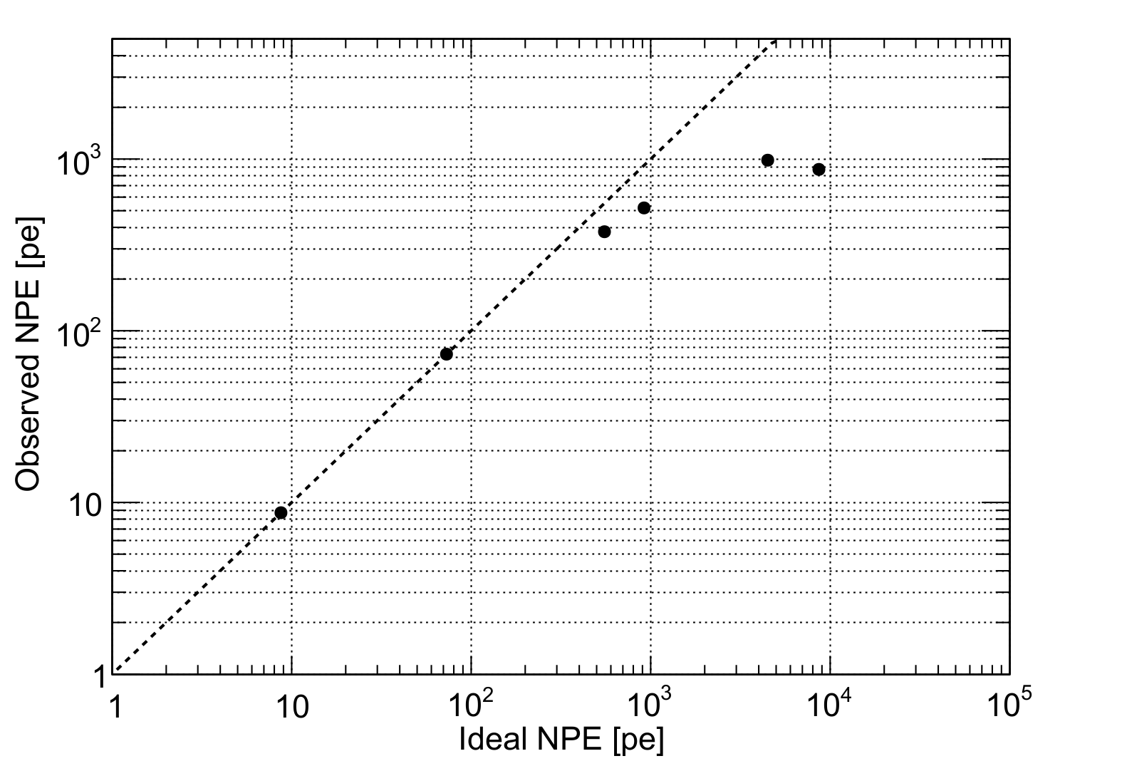
Fig. 23 Example charge linearity plot. Note that the dip at very high illumination is unusual.

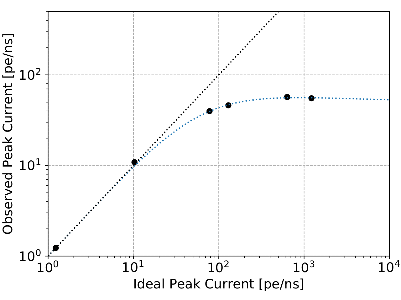
Fig. 24 Example current linearity plot. Note that the dip at very high illumination is unusual.

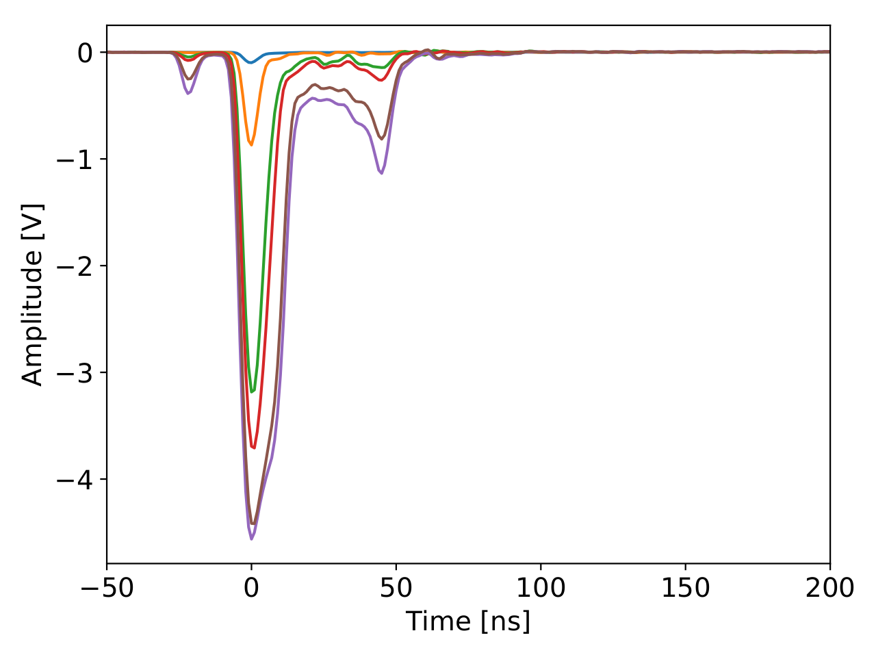
Fig. 25 Example average waveforms.