Shigeru Yoshida
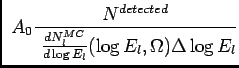
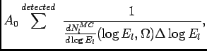
Expected event rate ![]() from a primary neutrino flux
from a primary neutrino flux ![]() at the earth surface can be obtained by
at the earth surface can be obtained by
where ![]() is energy of the secondary lepton such as
is energy of the secondary lepton such as ![]() ,
,
![]() is primary energy of neutrinos,
is primary energy of neutrinos,
![]() is number of secondary leptons produced
inside the earth and reaching to the IceCube volume,
and
is number of secondary leptons produced
inside the earth and reaching to the IceCube volume,
and ![]() is the effective area of the IceCube observatory.
The integral in the equation above accounts for the propagation
effect in the earth and obtained by resolving the relevant
transport equation [1]. This is equivalent to
the secondary lepton flux at the IceCube depth and pre-calculated
by JULIeT class like PropagatingNeutrinoFlux.java or
PropagatingAtmMuonFlux.java. An example is shown in
Figure 1.
is the effective area of the IceCube observatory.
The integral in the equation above accounts for the propagation
effect in the earth and obtained by resolving the relevant
transport equation [1]. This is equivalent to
the secondary lepton flux at the IceCube depth and pre-calculated
by JULIeT class like PropagatingNeutrinoFlux.java or
PropagatingAtmMuonFlux.java. An example is shown in
Figure 1.
![\includegraphics[width=.8\textwidth,clip=true]{gzk_4_4_85Deg}](img9.png) |
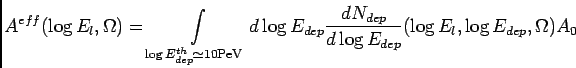
The effective area ![]() in Eq. 1
can be estimated by either the semi-analytical way [1]
or the full-brown MC. The semi-analytical method gives
in Eq. 1
can be estimated by either the semi-analytical way [1]
or the full-brown MC. The semi-analytical method gives
![]() as
as
 |
(2) |
By the full MC, the effective area will be given by
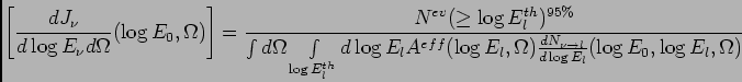
In this context the IceCube ``sensitivity'' for EHE neutrinos
can be obtained from a quasi-differential event rate in
neutrino model independent way. This approach has been widely
used in many other experiments (for example, see [2]).
The neutrino flux upper-bound with energy of ![]() from non-existence of signals is evaluated by putting
from non-existence of signals is evaluated by putting
![\begin{displaymath}
{dJ_\nu \over d\log{E_\nu}d\Omega}(\log{E_\nu}, \Omega)
=\le...
...mega}(\log{E_0}, \Omega)}\right]
\delta(\log{E_\nu}-\log{E_0})
\end{displaymath}](img24.png) |
(5) |